Introduction
What is geometric mechanics? At first blush, it is an approach to studying mechanics:
- classical Newtonian mechanics;
- Lagrangian mechanics;
- Hamiltonian mechanics;
- Nonholonomic mechanics.
Let us look briefly at each in turn.
Newtonian Mechanics
Classical mechanics \[ F = \ddt{t}{(mv)} = \ddt{t}{p} \]
- $m$ is the mass of the body;
- $v$ is the body's velocity;
- $F$ is the force acting;
- $p=mv$ is the momentum.
Newtonian Mechanics
Classical mechanics - clarifications \[ \underbrace{F}_{{\color{red}{\textrm{what is a force?}}}} = \underbrace{\ddt{t}{\overbrace{(mv)}^{{\color{red}{\textrm{what is mass? velocity?}}}}}}_{{\color{red}{\textrm{what is the rate of change of velocity?}}}} = \overbrace{\ddt{t}{p}}^{{\color{red}{\textrm{what is momentum?}}}} \]
- $m$ is the mass of the body;
- $v$ is the body's velocity;
- $F$ is the force acting;
- $p=mv$ is the momentum.
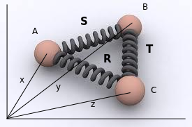
An Example - springs & masses
 \begin{align*}
A \ddot{x} &= -S(x-y) - R(x-z) \\
B \ddot{y} &= -S(y-x) - T(y-z) \\
C \ddot{z} &= -R(z-x) - T(z-y)
\end{align*}
\begin{align*}
A \ddot{x} &= -S(x-y) - R(x-z) \\
B \ddot{y} &= -S(y-x) - T(y-z) \\
C \ddot{z} &= -R(z-x) - T(z-y)
\end{align*}
An Example - springs & masses
\begin{align*}
\dfrac{d\,}{dt}
\begin{bmatrix}
A & 0 & 0\\0 & B & 0\\0 & 0 & C
\end{bmatrix}
\begin{bmatrix}
\dot{x}\\\dot{y}\\\dot{z}
\end{bmatrix}
&=
-
\begin{bmatrix}
+S+R & -S & -R\\
-S & +S+T & -T\\
-R & -T & +R+T
\end{bmatrix}
\begin{bmatrix}
x\\y\\x
\end{bmatrix}
\\
\dfrac{d\,}{dt} \mathbf{M} \dot{\mathbf{q}} &= -\mathbf{Q} \mathbf{q}
\end{align*}
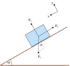
What is a force?
A Force is something we integrate over a path to compute Work done.
 \begin{align*}
W &= \int\limits_{\sigma}^{} \ip{F}{d \sigma}
\end{align*}
\begin{align*}
W &= \int\limits_{\sigma}^{} \ip{F}{d \sigma}
\end{align*}
What is a force?
A Force is a differential 1-form.
- a force $F$ is conservative if the line integral \( \displaystyle\oint_{\sigma}^{} \ip{F}{\D{\sigma}} \) vanishes for all closed loops.
- a 1-form $F$ is exact if it integrates to zero along all closed loops, in which case \( F = \D{f} \) for some smooth function $f$.
An example - spring force
Let's compute the exterior derivative of the force 1-form $F$ for the spring-mass system:
\begin{align*} F &= \sum_i (\mathbf{Qq})_i \D{\mathbf{q}}_i = \sum_{i, j} \mathbf{Q}_{ij}\mathbf{q}_j \D{\mathbf{q}}_i \\ \D{F} &= \sum_{i, j} \mathbf{Q}_{ij} \D{\mathbf{q}}_j \wedge \D{\mathbf{q}}_i = 0 \end{align*}
An example - spring force
This shows $F$ is *closed*. It is exact since every closed 1-form on $\R^n$ is exact. We compute, for the path $\sigma(t) = t \mathbf{q},$\begin{align*} f(\mathbf{q}) &= \wint{\mathbf{0}}{\mathbf{q}} \ip{F(\sigma(t))}{\dot{\sigma}(t)} \D t = \wint{0}{1} \ip{F(t \mathbf{q})}{\mathbf{q}} \D t\\ &= - \wint{0}{1} \ip{\mathbf{Qq}}{\mathbf{q}} t \D t = - \wint{0}{1} t \D t \times \ip{\mathbf{Qq}}{\mathbf{q}} = - \frac{1}{2} \ip{\mathbf{Qq}}{\mathbf{q}}. \end{align*}
By definition $U = -f$ is the potential energy of the system.
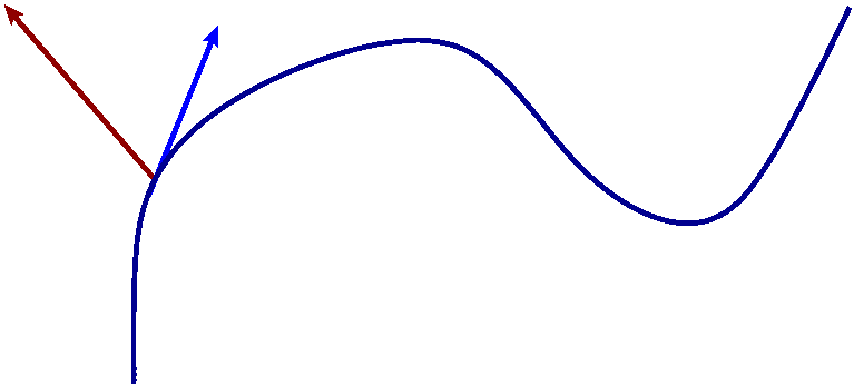
What is a velocity?
- The velocity of a point with position $p(t)$ at time $t$ is $\dot{p}(t)$.
- We measure velocity by a measuring rod, $f$ (a scalar valued function). $$\dot{f}(t) = \ddt{t}{} f \circ p(t)$$
 |
| How to measure velocity. |
What is a velocity?
We need to do calculus. To do calculus, we need differentiable manifolds.
What is a velocity?
We need to do calculus. To do calculus, we need differentiable manifolds.
- A differentiable manifold $M$ is a (Hausdorff) topological space, an open covering $C=\set{U}$, and homeomorphisms $\phi_U : U \to \R^n$.
- The homeomorphisms $\phi_U$ satisfy: $$\phi_U \circ \phi_V^{-1} : \phi_V(U \cap V) \to \phi_U(U \cap V)$$ is a diffeomorphism for all $U, V \in C$.
 |
| Coordinate charts |
Examples of manifolds
- $\R^n$
- $\sphere{n} \subset \R^{n+1}$ (the unit sphere)
- The group of $n \times n$ matrices of non-zero determinant, $\GL{\R^n}$.
- The group of solid rotations.
- The set of all lines in $\R^3$.
A worked example
Let $\sphere{2} \subset \R^3$ be the unit sphere.
- regular level set;
- stereographic projection;
- graph.
A worked example
Let $A$ be the set of all lines $\R^3$.
-
each line $\ell$ can be written as $\ell = \set{p + t v \st t \in \R}$ where:
- $v$ has unit length;
- $p$ and $v$ are orthogonal;
- $v$ is unique up to a change of sign (= orientation of the line).
- $A \simeq \set{ (v, p) \in \R^3 \times \R^3 \st \norm{v}=1, \ip{v}{p}=0 }/\sim.$
Vector fields and differential forms
Let $M$ be a manifold with a coordinate system $x : U \subset M \to \R^n$.
- We get functions $x_i$ defined on $U$;
- We get vector fields $$\didi{}{x_i}$$
- We get differential forms $$\D{x_i}$$
- Each vector field $V$ on $M$ has $$V|U = V_1(x) \didi{}{x_1} + \cdots + V_n(x) \didi{}{x_n}$$
- Each differential 1-form $F$ has $$F|U = F_1(x) \D{x_1} + \cdots + F_n(x) \D{x_n}$$
Vector fields and differential forms
We compute that \begin{align*} \ip{\D{x_i}}{\didi{}{x_j}} &= \didi{x_i}{x_j} = \delta_{ij} \\ \ip{\D{x_i}}{V} &= \lieder{V}{x_i} = \sum_j V_j \times \ip{\D{x_i}}{\didi{}{x_j}} = V_i \\ \ip{F}{V} &= \sum_i F_i(x) V_i(x). \end{align*}